Square Root in Verilog
The square root is useful in many circumstances, including statistics, graphics, and signal processing. In this how to, we’re going to look at a straightforward digit-by-digit square root algorithm for integer and fixed-point numbers. There are lower-latency methods, but this one is simple, using only subtraction and bit shifts. New to Verilog maths? Check out my introduction to Numbers in Verilog.
Share your thoughts with @WillFlux on Mastodon or Twitter. If you like what I do, sponsor me. 🙏
Source
The SystemVerilog designs featured in this post are available from the Project F Library under the open-source MIT licence: build on them to your heart’s content. The rest of the blog content is subject to standard copyright restrictions: don’t republish it without permission.
Getting Radical
The square root of a number is a second number that multiplied by itself produces the first number. If b is the square root of a, then the following are different ways of representing their relationship:
b² = ab = a1/2b = √a
The square root is usually represented with the radical sign √.
Let’s look at a few concrete examples:
√4 = 2√100 = 10√2 ≈ 1.41421√3 ≈ 1.73205
Most square roots are irrational, so we only get an approximate answer algorithmically. However, the good news is that our method will provide an exact solution if one exists.
We’re only going to consider the positive root in this post, but there is also a negative root. For example, the square roots of 4 are +2 and -2.
Triangles
Pythagoras’s theorem is a fundamental equation in geometry. For a right-angled triangle, the area of the square of the hypotenuse is equal to the sum of the areas of the squares on the other two sides.
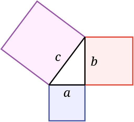
a² + b² = c²
Finding c is a common problem in computer graphics, which means solving √(a² + b²).
For 3D modelling, it’s common to need the reciprocal of c.
Diagram courtesy of Wikipedia under the Creative Commons Attribution-Share Alike licence.
The Long Route
So far, so (probably) familiar. However, you’re unlikely to have calculated square roots by hand. Superficially, square roots seem too hard to do manually, but the approach is almost the same as long division. I won’t go into the mathematics here, but Wikipedia has a decent write up: methods of computing square roots. Instead, we’ll take a simple example, then turn it into a Verilog algorithm.
Example: √1111001
The number we’re finding the root of is known as the radicand.
For our example, the radicand is 1111001 (121 in decimal).
Our algorithm works with pairs of digits. Before we begin our calculation, we need to split the radicand into pairs starting with the least significant. Thus 1111001 becomes 01 11 10 01.
     1  0  1  1     Our answer: one digit for each pair of digits in the radicand
    ———————————
   √01 11 10 01     Our radicand

    01              Bring down the most significant pair
  - 01              Subtract 01
    ——
    00              Our answer is NOT negative, so our first answer digit is 1

    00 11           Bring down the next pair of digits and append to previous result
  - 01 01           Append 01 to our existing answer, 1, and subtract it
    —————
    11 00           Our result is negative, so our second answer digit is 0
                    We discard the result because it's negative

    00 11 10        Keep the existing digits, 00 11, and append the next pair
  -    10 01        Append 01 to our existing answer, 10, and subtract it
    ————————
       01 01        Our answer is NOT negative, so our next answer digit is 1

       01 01 01     Bring down the next pair of digits and append to previous result
    -  01 01 01     Append 01 to our existing answer, 101, and subtract it
       ————————
             00     Our answer is NOT negative, so our next answer digit is 1
There are no more pairs of digits, and the result of our last step is 0, so our answer is exact:
√1111001 = 1011 or in decimal √121 = 11.
We’ll look at what happens for irrational roots, such as √2, when we come to fixed-point numbers.
Algorithm Implementation
To make our algorithm usable on an FPGA, we need to turn the steps into simple operations we can represent in Verilog. The main change is using shifts to select numbers to work on. We’ll use four registers in our algorithm:
- X - input radicand we want the square root of
- A - holds the current value we’re working on
- T - result of sign test
- Q - the square root
Input: X=01111001 (decimal 121)

Step  A         X         T         Q       Description
——————————————————————————————————————————————————————————————————————————————
      00000000  01111001  00000000  0000    Starting values.

1     00000001  11100100                    Left shift X by two places into A.
                          00000000          Set T = A - {Q,01}: 01 - 01.
                                    0000    Left shift Q.
      00000000                      0001    Is T≥0? Yes. Set A=T and Q[0]=1.

2     00000011  10010000                    Left shift X by two places into A.
                          11111100          Set T = A - {Q,01}: 11 - 101.
                                    0010    Left shift Q.
                                            Is T≥0? No. Move to next step.

3     00001110  01000000                    Left shift X by two places into A.
                          00000101          Set T = A - {Q,01}: 1110 - 1001
                                    0100    Left shift Q.
      00000101                      0101    Is T≥0? Yes. Set A=T and Q[0]=1.

4     00010101  00000000                    Left shift X by two places into A.
                          00000000          Set T = A - {Q,01}: 10101 - 10101.
                                    1010    Left shift Q.
      00000000                      1011    Is T≥0? Yes. Set A=T and Q[0]=1.
——————————————————————————————————————————————————————————————————————————————

Output: Q=1010 (decimal 11), R=0 (remainder taken from final A).
Verilog Module
Our Verilog design uses the above algorithm, but you can configure the width of the radicand. WIDTH must be a multiple of two, for example, when working with seven binary digits, you must set the width to eight.
Project F Library source: [sqrt_int.sv].
module sqrt_int #(parameter WIDTH=8) (      // width of radicand
    input wire logic clk,
    input wire logic start,             // start signal
    output     logic busy,              // calculation in progress
    output     logic valid,             // root and rem are valid
    input wire logic [WIDTH-1:0] rad,   // radicand
    output     logic [WIDTH-1:0] root,  // root
    output     logic [WIDTH-1:0] rem    // remainder
    );

    logic [WIDTH-1:0] x, x_next;    // radicand copy
    logic [WIDTH-1:0] q, q_next;    // intermediate root (quotient)
    logic [WIDTH+1:0] ac, ac_next;  // accumulator (2 bits wider)
    logic [WIDTH+1:0] test_res;     // sign test result (2 bits wider)

    localparam ITER = WIDTH >> 1;   // iterations are half radicand width
    logic [$clog2(ITER)-1:0] i;     // iteration counter

    always_comb begin
        test_res = ac - {q, 2'b01};
        if (test_res[WIDTH+1] == 0) begin  // test_res ≥0? (check MSB)
            {ac_next, x_next} = {test_res[WIDTH-1:0], x, 2'b0};
            q_next = {q[WIDTH-2:0], 1'b1};
        end else begin
            {ac_next, x_next} = {ac[WIDTH-1:0], x, 2'b0};
            q_next = q << 1;
        end
    end

    always_ff @(posedge clk) begin
        if (start) begin
            busy <= 1;
            valid <= 0;
            i <= 0;
            q <= 0;
            {ac, x} <= {{WIDTH{1'b0}}, rad, 2'b0};
        end else if (busy) begin
            if (i == ITER-1) begin  // we're done
                busy <= 0;
                valid <= 1;
                root <= q_next;
                rem <= ac_next[WIDTH+1:2];  // undo final shift
            end else begin  // next iteration
                i <= i + 1;
                x <= x_next;
                ac <= ac_next;
                q <= q_next;
            end
        end
    end
endmodule
To use the module, set WIDTH to the correct number of bits and input rad to the radicand. To begin the calculation set start high for one clock. The valid signal indicates when the output data is valid; you can then read the results from root and rem. The calculation takes one cycle for each pair of bits in the radicand, so a 16-bit radicand would take eight cycles. The busy signal is high during calculation.
The Verilog itself is straightforward. The algorithm is in the always_comb block, though we start with the initial shift already in place. The always_ff block sets up the initial values, then runs the algorithm for the number of digits in the root.
Testing
The following Vivado test bench exercises the module. A Verilator test bench will be added in due course.
Project F Library source: [xc7/sqrt_int_tb.sv].
module sqrt_int_tb();

    parameter CLK_PERIOD = 10;
    parameter WIDTH = 8;

    logic clk;
    logic start;             // start signal
    logic busy;              // calculation in progress
    logic valid;             // root and rem are valid
    logic [WIDTH-1:0] rad;   // radicand
    logic [WIDTH-1:0] root;  // root
    logic [WIDTH-1:0] rem;   // remainder

    sqrt_int #(.WIDTH(WIDTH)) sqrt_inst (.*);

    always #(CLK_PERIOD / 2) clk = ~clk;

    initial begin
        $monitor("\t%d:\tsqrt(%d) =%d (rem =%d) (V=%b)", $time, rad, root, rem, valid);
    end

    initial begin
                clk = 1;

        #100    rad = 8'b00000000;  // 0
                start = 1;
        #10     start = 0;

        #50     rad = 8'b00000001;  // 1
                start = 1;
        #10     start = 0;

        #50     rad = 8'b01111001;  // 121
                start = 1;
        #10     start = 0;

        #50     rad = 8'b01010001;  // 81
                start = 1;
        #10     start = 0;

        #50     rad = 8'b01011010;  // 90
                start = 1;
        #10     start = 0;

        #50     rad = 8'b11111111;  // 255
                start = 1;
        #10     start = 0;

        #50     $finish;
    end
endmodule
The output looks like this (V=1 indicates the result is valid):
  0:    sqrt(  x) =  x (rem =  x) (V=x)
100:    sqrt(  0) =  x (rem =  x) (V=0)
140:    sqrt(  0) =  0 (rem =  0) (V=1)
160:    sqrt(  1) =  0 (rem =  0) (V=0)
200:    sqrt(  1) =  1 (rem =  0) (V=1)
220:    sqrt(121) =  1 (rem =  0) (V=0)
260:    sqrt(121) = 11 (rem =  0) (V=1)
280:    sqrt( 81) = 11 (rem =  0) (V=0)
320:    sqrt( 81) =  9 (rem =  0) (V=1)
340:    sqrt( 90) =  9 (rem =  0) (V=0)
380:    sqrt( 90) =  9 (rem =  9) (V=1)
400:    sqrt(255) =  9 (rem =  9) (V=0)
440:    sqrt(255) = 15 (rem = 30) (V=1)
Fixed-Point Roots
In a previous recipe, we looked at Fixed Point Numbers in Verilog. It turns out that supporting fixed-point square roots is straightforward: we just run more iterations to account for the fractional digits. Unlike with division, there’s no possibility of overflow, as the root of a radicand greater than 1 is always smaller than the radicand itself.
This new version of the sqrt module adds a parameter FBITS for the number of fractional bits in the radicand (FBITS must be a multiple of two). For example, if we want to calculate √2 using Q8.8 format (eight integer and eight fractional bits), we set WIDTH=16 and FBITS=8. The only change within the module is for ITER, which now accounts for fractional bits. For a Q8.8 radicand, we now perform (16+8)/2 = 12 iterations, generating four more bits for the root.
Project F Library source: [sqrt.sv].
module sqrt #(
    parameter WIDTH=8,  // width of radicand
    parameter FBITS=0   // fractional bits (for fixed point)
    ) (
    input wire logic clk,
    input wire logic start,             // start signal
    output     logic busy,              // calculation in progress
    output     logic valid,             // root and rem are valid
    input wire logic [WIDTH-1:0] rad,   // radicand
    output     logic [WIDTH-1:0] root,  // root
    output     logic [WIDTH-1:0] rem    // remainder
    );

    logic [WIDTH-1:0] x, x_next;    // radicand copy
    logic [WIDTH-1:0] q, q_next;    // intermediate root (quotient)
    logic [WIDTH+1:0] ac, ac_next;  // accumulator (2 bits wider)
    logic [WIDTH+1:0] test_res;     // sign test result (2 bits wider)

    localparam ITER = (WIDTH+FBITS) >> 1;  // iterations are half radicand+fbits width
    logic [$clog2(ITER)-1:0] i;            // iteration counter

    always_comb begin
        test_res = ac - {q, 2'b01};
        if (test_res[WIDTH+1] == 0) begin  // test_res ≥0? (check MSB)
            {ac_next, x_next} = {test_res[WIDTH-1:0], x, 2'b0};
            q_next = {q[WIDTH-2:0], 1'b1};
        end else begin
            {ac_next, x_next} = {ac[WIDTH-1:0], x, 2'b0};
            q_next = q << 1;
        end
    end

    always_ff @(posedge clk) begin
        if (start) begin
            busy <= 1;
            valid <= 0;
            i <= 0;
            q <= 0;
            {ac, x} <= {{WIDTH{1'b0}}, rad, 2'b0};
        end else if (busy) begin
            if (i == ITER-1) begin  // we're done
                busy <= 0;
                valid <= 1;
                root <= q_next;
                rem <= ac_next[WIDTH+1:2];  // undo final shift
            end else begin  // next iteration
                i <= i + 1;
                x <= x_next;
                ac <= ac_next;
                q <= q_next;
            end
        end
    end
endmodule
And we can create a simple Vivado test bench for it.
Project F Library source: [xc7/sqrt_tb.sv].
module sqrt_tb();

    parameter CLK_PERIOD = 10;
    parameter WIDTH = 16;
    parameter FBITS = 8;
    parameter SF = 2.0**-8.0;  // Q8.8 scaling factor is 2^-8

    logic clk;
    logic start;             // start signal
    logic busy;              // calculation in progress
    logic valid;             // root and rem are valid
    logic [WIDTH-1:0] rad;   // radicand
    logic [WIDTH-1:0] root;  // root
    logic [WIDTH-1:0] rem;   // remainder

    sqrt #(.WIDTH(WIDTH), .FBITS(FBITS)) sqrt_inst (.*);

    always #(CLK_PERIOD / 2) clk = ~clk;

    initial begin
        $monitor("\t%d:\tsqrt(%f) = %b (%f) (rem = %b) (V=%b)",
                    $time, $itor(rad*SF), root, $itor(root*SF), rem, valid);
    end

    initial begin
                clk = 1;

        #100    rad = 16'b1110_1000_1001_0000;  // 232.56250000
                start = 1;
        #10     start = 0;

        #120    rad = 16'b0000_0000_0100_0000;  // 0.25
                start = 1;
        #10     start = 0;

        #120    rad = 16'b0000_0010_0000_0000;  // 2.0
                start = 1;
        #10     start = 0;
        #120    $finish;
    end
endmodule
NB. I have tested with a wide range of roots, but only show a few here to keep the example managable.
The output looks like this (V=1 indicates the result is valid):
  0:    sqrt(0.000000)   = xxxxxxxxxxxxxxxx (0.000000)  (rem = xxxxxxxxxxxxxxxx) (V=x)
100:    sqrt(232.562500) = xxxxxxxxxxxxxxxx (0.000000)  (rem = xxxxxxxxxxxxxxxx) (V=0)
220:    sqrt(232.562500) = 0000111101000000 (15.250000) (rem = 0000000000000000) (V=1)
230:    sqrt(0.250000)   = 0000111101000000 (15.250000) (rem = 0000000000000000) (V=0)
350:    sqrt(0.250000)   = 0000000010000000 (0.500000)  (rem = 0000000000000000) (V=1)
360:    sqrt(2.000000)   = 0000000010000000 (0.500000)  (rem = 0000000000000000) (V=0)
480:    sqrt(2.000000)   = 0000000101101010 (1.414062)  (rem = 0000000000011100) (V=1)
1.01101010 is the correct result for √2 using eight fractional bits. Wolfram Alpha provides a quick way to check binary square roots, for example: √2 to base 2.
The smallest value the Q8.8 format can represent is 1/256 or ~0.004 in decimal; if you want a more accurate result, you need to use more fractional bits.
What’s Next?
That wraps up this FPGA recipe, but you might like to check out Division in Verilog or Sine & Cosine.